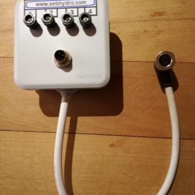
Test box for 3- and 4-wire sensor
99,00€
89,10€ inc. tax
82,50€
74,25€ excl. tax

0,00€ inc. tax 0,00€ excl. tax
Details
Hydraulic training : The basics Vol 1
55,00€ inc. tax 52,13€ excl. tax
Details
Hydraulic training : The basics Vol 1
55,00€ inc. tax 52,13€ excl. tax
Details
1- Open loop
55,00€ inc. tax 52,13€ excl. tax
Details
Test box for 3- and 4-wire sensor
99,00€
89,10€ inc. tax
82,50€
74,25€ excl. tax
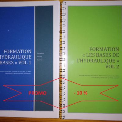
Formation hydraulique "les bases" vol 1&2
110,00€
99,00€ inc. tax
104,27€
93,84€ excl. tax
2- closed loop
55,00€ inc. tax 52,13€ excl. tax
Details
3- PID regulator
55,00€ inc. tax 52,13€ excl. tax
Details
55,00€ inc. tax 52,13€ excl. tax
Details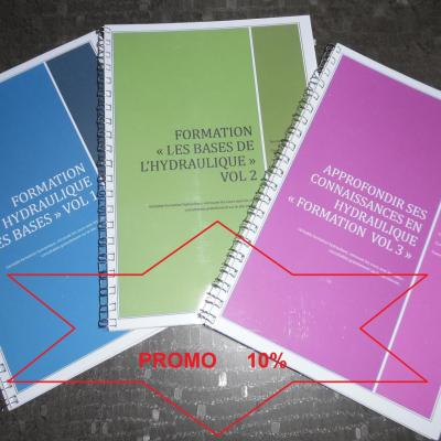
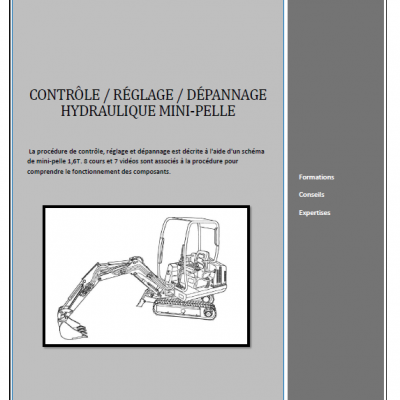
165,00€
148,50€ inc. tax
156,40€
140,76€ excl. tax
The proportional gain P : Speed

2 - The different settings
Integral corrector I : Precision

Ramps
The derivate corrector D : Stability, anticipation

3 - Important concepts
PID Parameter Tuning Method
4- Hydraulic rigidity
Hydraulic stiffness :
5-Natural frequency
Natural frequency of a mechanical system :

55,00€ inc. tax 52,13€ excl. tax
DetailsNatural frequency of a piston pump :
55,00€ inc. tax 52,13€ excl. tax
DetailsComments
-
 Bonjour
Très bien, simple, clair et efficace
Merci
Add a comment